The Naive Bayes Classifier

I’ve needed to derive and use the naive Bayes classifier a few times over the past years, so for my own reference I’m writing down here all of the steps in the derivation of the classifier along with a couple of example use cases so that I can refresh my memory as needed.

The Problem

The problem we are solving is as follows: Imagine a training dataset described by \(n\) features, \(F_1, F_2, ... F_n\). This training set is classified by hand into one of the classes \(C\). The classifier needs to, given a new set of \(n\) features, predict which of the classes \(C\) the new data corresponds to. That is, we want to calculate \(P(C\vert F_1\cap F_2\cap ... \cap F_n)\).

The Naive Bayesian Probabalistic Model

In the case where there are millions of features, or many values that each feature can take, looking up \(P(C\vert F_1\cap F_2\cap ... \cap F_n)\) in probability tables is not feasible, so we turn to Bayes rule:

\[P(C\vert F_1\cap F_2\cap ... \cap F_n)=\frac{P(F_1\cap F_2\cap ... \cap F_n\vert C)P(C)}{P(F_1\cap F_2\cap ... \cap F_n)}=\frac{P(C\cap F_1\cap ... \cap F_n)}{P(F_1\cap F_2\cap ... \cap F_n)}\]

Only the numerator of the fraction is interesting for classification, the denominator is just a constant number that depends on the particular set of features chosen, so:

\[P(C\vert F_1\cap F_2\cap ... \cap F_n)\propto P(C\cap F_1\cap ... \cap F_n)\]

We can make the numerator that remains more tractable by noting that we can break down a bunch of joint probabilities through repeated application of the definition of conditional probability. Concretely, for the case of four variables, \(A_1\) through \(A_4\):

\[P(A_1\cap A_2\cap A_3\cap A_4)=P(A_4\vert A_3\cap A_2\cap A_1)P(A_3\vert A_2\cap A_1)P(A_2\vert A_1)P(A_1)\]

More generally, for the case of \(n\) variables:

\[P(A_1\cap ...\cap A_n)= P(A_1)P(A_2\vert A_1)P(A_3\vert A_2\cap A_1)...P(A_n\vert A_1\cap A_2\cap ... \cap A_{n-1})\]

We use this to write for our problem: \(P(C\cap F_1\cap ... \cap F_n)=P(C)P(F_1\vert C)P(F_2\vert C\cap F_1)...P(F_n\vert C\cap F_1\cap F_2\cap ...\cap F_{n-1})\)

Now we need to make the assumption that each of the features \(F_i\) is conditionally independent of all of the other features. That is, \(P(F_i\vert C\cap F_j)=P(F_i\vert C)\) and \(P(F_i\vert C\cap F_j\cap F_l)=P(F_i\vert C)\) and so on. This removes all of the conditions above and we can simplify the previous equation to

\[P(C\vert F_1\cap F_2\cap ... \cap F_n)\propto P(C)P(F_1\vert C)P(F_2\vert C)...P(F_n\vert C) = P(C)\prod_{i=1}^nP(F_i\vert C)\]

The Binary Classification Problem

So far we have derived the naive Bayes probability model, we need to add a decision rule to make a classifier. One very common choice is just to pick the most probable class (the maximum a posteriori or MAP decision rule). In general, we do not expect the features to be independent, but the naive Bayesian model is still of a surprising amount of use. In general we don’t expect the values for the probabilities of class membership to be accurate if the features are dependent, but as long as they’re in the correct order the MAP decision rule will still return the correct.

Imagine now a situation where, for a given set of \(n\) features \(F_1, F_2, F_3,...,F_n\) we wish to decide whether a particular entry belongs to a class (\(C\)) or does not (\(\bar{C}\)). We begin by defining the likelihood ratio:

\[\frac{P(C\vert F_1\cap F_2\cap ... \cap F_n)}{P(\bar{C}\vert F_1\cap F_2\cap ... \cap F_n)}=\frac{P(C)}{P(\bar{C})}\frac{\prod_{i=1}^nP(F_i\vert C)}{\prod_{i=1}^nP(F_i\vert \bar{C})}\]

Here, \(P(C)\) and \(P(\bar{C})\) represent our knowledge of the prior probabilities. This prior probability distribution might be based on our knowledge of frequencies in the larger population, or on frequency in the training set. It is also important to note that the product is carried out over all features, including those that are negative in the sample we’re considering.

If the likelihood ratio is greater than 1, the naive Bayesian classifier predicts that a given entry belongs to class \(C\). In practice, there are frequently many thousands of features and the probabilities of any given feature being present may be very small, so we work in terms of the log likelihood

\[\ln \frac{P(C\vert F_1\cap F_2\cap ... \cap F_n)}{P(\bar{C}\vert F_1\cap F_2\cap ... \cap F_n)}=\ln \frac{P(C)}{P(\bar{C})}+\ln\frac{\prod_{i=1}^nP(F_i\vert C)}{\prod_{i=1}^nP(F_i\vert\bar{C})}\]

Worked Example: Sentiment Analysis

Imagine that you have the following set of messages about a mobile phone

A table of example tweets and their classifications

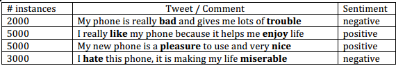
We wish to be able to automatically classify new messages that we receive either as having a positive or negative sentiment. From the overall population, \(P(+)=5000/10000=0.5\) and \(P(-)=5000/10000=0.5\). We can now calculate the conditional probabilities for each word being in a positive and negative message.

Conditional probabilities of words being in positive and negative sentiment tweets.

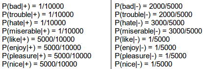
Note here that we have employed ‘smoothing’ or ‘pseudocounting’. Where a term doesn’t appear in a given class (e.g. the word hate appears in no positive messages) we don’t want to return a zero as it sends the likelihood calculation haywire. Instead we make it the smallest possible number. Now consider trying to automatically classify the following message

A tweet reading ‘I take no pleasure in using this phone. It is nothing but trouble’

The prefactors outside the fromt of the likelihood ratio cancel out (\(P(+)=P(-)\)), and multiplying out the remaining products gives

Conditional probability calculation on the tweet.

I don’t know which way this works out, but it highlights one big weakness with naive Bayes. That is that we have assumed the message is a bag of words, where their relative positions are unimportant. For example, the presence of no in front of pleasure makes this a negative statement that naive Bayes interprets incorrectly.